I’m launching an app for saving web articles to read later. Well, I’m launching a client for a read-later service—a client I started developing because the first-party apps didn’t support a particular feature. A feature that was added to the official apps a couple days after I started working on mine. But since then I’ve spent chunks of free time over the last month developing this app, which is now in beta.
Let’s back up.
Almost seven weeks ago, Matt Birchler published a blog post with the headline, “I built the read later app I’d always wanted”, in which he publicly released Quick Reads. I’d actually had early access to the web app and iOS TestFlight beta since February, and had been really enjoying it. I still had articles saved in Matter that I was going back to read sometimes—and some really long ones I was sending to Instapaper to read on my Kobo—but for the most part everything I’ve saved new since then has gone into Quick Reads. The one thing I was really missing was the ability to pick up an article where I left off if I didn’t read it in one sitting. There was a time not that long ago where I would’ve just put in a feature request to the developer and then seen if anything ever came of it. But Quick Reads isn’t just a web and iOS app—it’s also a well-documented API that covers pretty much everything the apps do. And I’ve increasingly been throwing Claude Code at problems and itches to scratch, so a couple weeks after Matt’s announcement post, I decided to see what I could whip up using his API. On the 7th of May, I made the first commit on an Xcode project I called “Slow Reads”.
The next evening, I was inspired to post about my decision-making paradigm on Mastodon:
Quick Reads (https://quickreads.app) is great, but I wish it would remember where I am in an article.
Year-ago me (hypothetically): Send @matt_birchler a feature request. Wait.
2026 me: Fire up Claude Code.
15 minutes after I published that, Matt replied to say that he was already working on that feature by popular request, and less than 9 hours later—the middle of the night my time—he followed up to say that it had shipped.[1] By then, though, I had already tasted the potential of developing the read-later app I’ve always wanted.
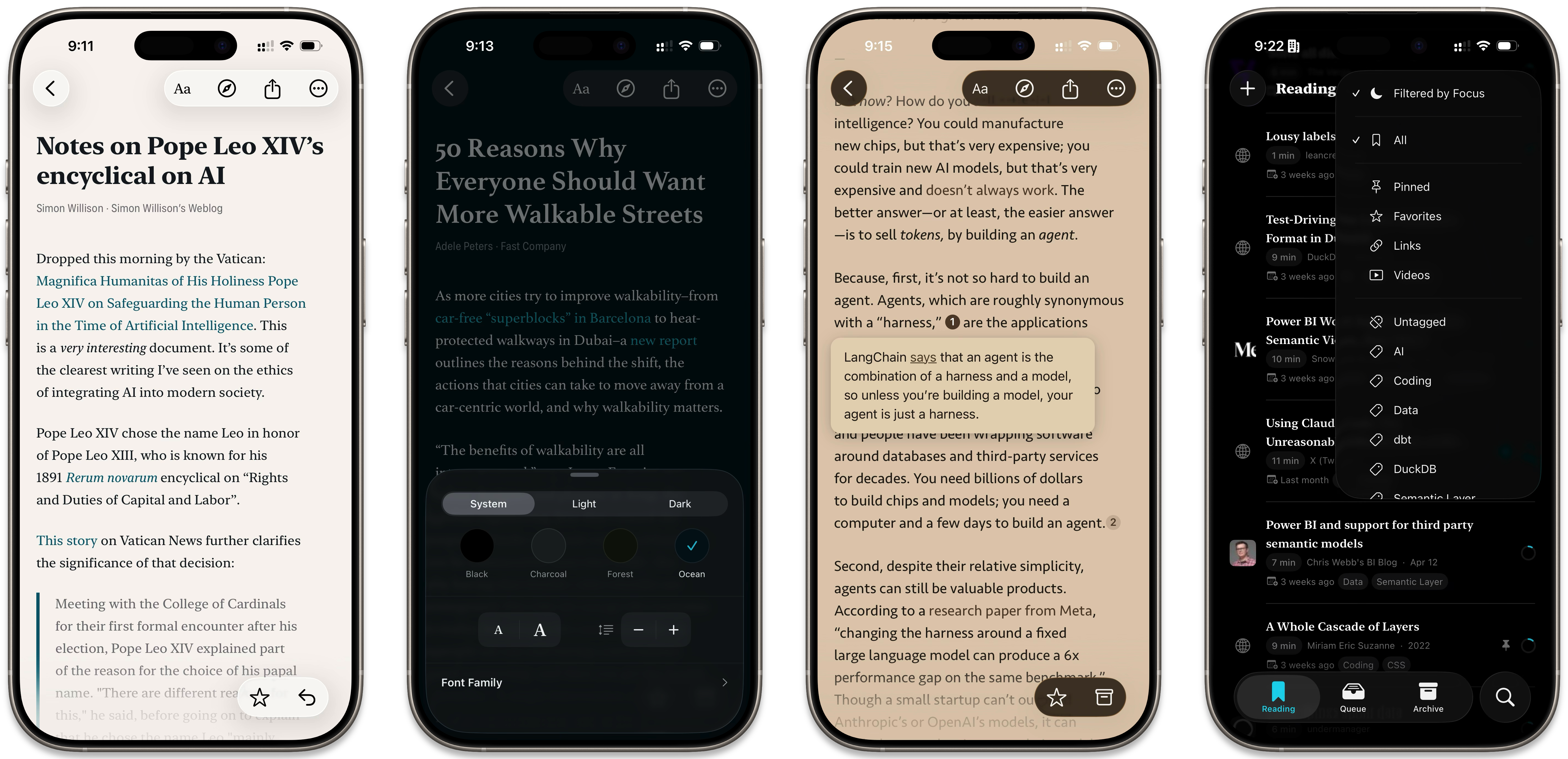
I’ve tried almost every big read-later service that’s come along: from the OG, Instapaper, to the early competitors, Pocket and Readability, to the new cool kids on the block, Matter and Readwise Reader. So I’ve taken inspiration from the things I liked about all of them. Matter has lots of font choices and several great dark and light themes that can be synced to or independent of the system appearance. GoodLinks is the only one I know of with Focus filters for your tags. Instapaper is the only one I remember parsing footnotes and displaying them as popovers.
At least at time of writing, Quick Reads doesn’t have any first-party support for importing from any other services. For the most part, it was actually a bit of a relief to just start fresh, without the four thousand articles I’d migrated from one service to another over the years. But I realized that Matter has also documented its API (which was not true the last time I was trying to automate anything related to Matter), and that I did at least want to bring over a subset of what was in Matter. I ended up setting up an import flow with granular control over importing the queue, archive, favorites, and highlights, with the full article contents where available.
For myself, I archived everything except the handful of articles I wanted to migrate[2] and imported those along with anything I’d highlighted or marked as a favorite, so now I have those for posterity without the entire overgrown library of stuff I’d saved and maybe or maybe not ever gotten around to reading.
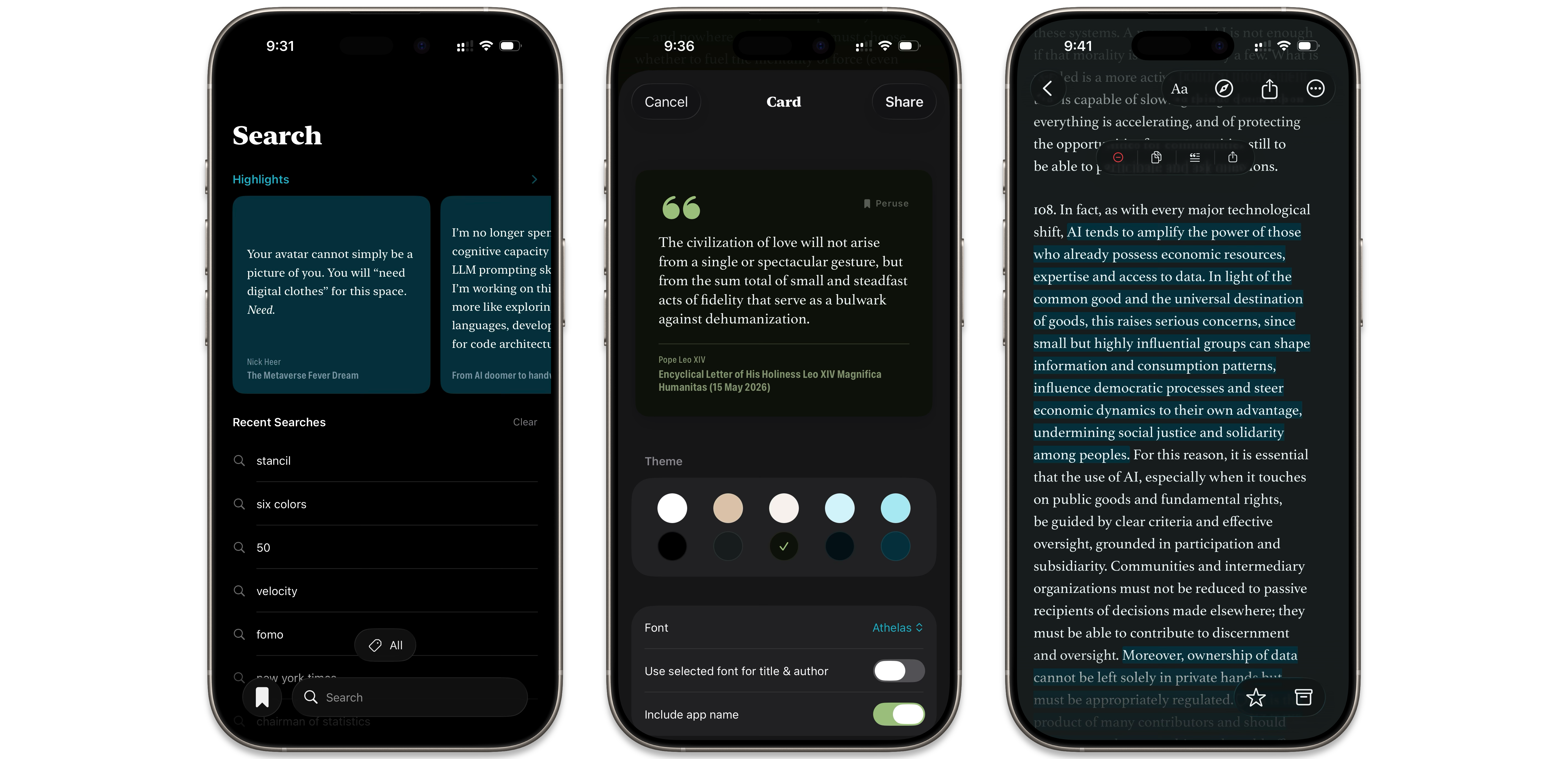
I also got really into building around highlights, including a carousel in the Search tab and an interface for sharing “textshot”-style images of snippets you’ve highlighted (or selected), with customization for the font and color scheme.
One feature that I really like about Quick Reads is an auto-archive setting to automatically clean up articles older than 7, 14, or 28 days (from the date they were saved). But with the (initial) premise of my app being a client that lets you pick up where you left off, I wanted it to skip articles I was in the middle of, regardless of their age. So I implemented my own version of this feature that skips in-progress articles. Then I took it a step further and introduced the idea of pinned articles,[3] which can have two uses: to keep articles at the top of the queue, and/or to keep them from being auto-archived when they would otherwise age out. Of course, this actually requires disabling the feature in the Quick Reads settings so it doesn’t go ahead and archive the ones you wanted skipped.
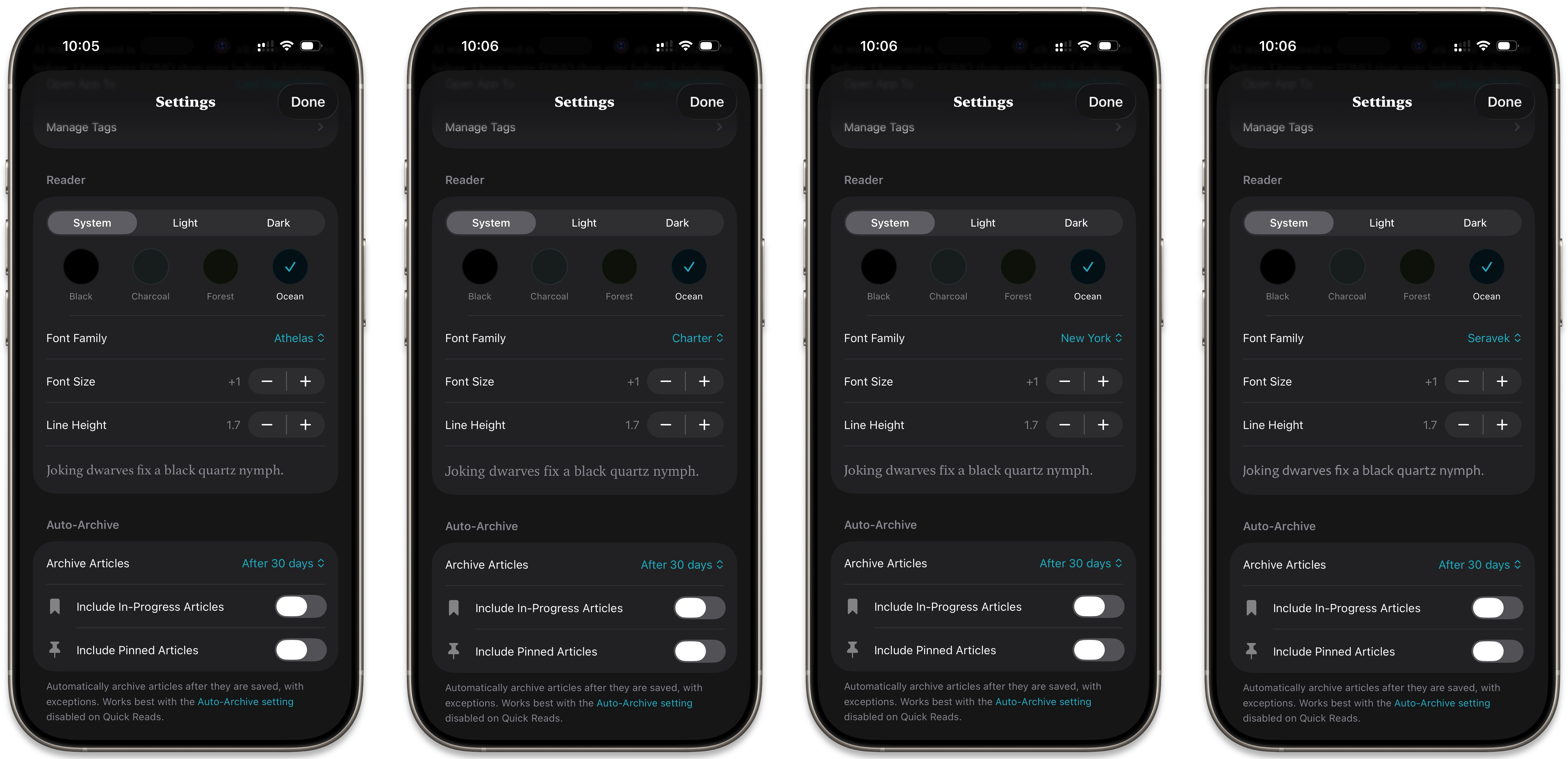
The last thing I’ll mention that was kind of fun was figuring out the preview text. When you bring up the appearance settings in the reader view, they are overlaid on the article so you can see the effects of your changes. In the Settings screen, I added preview text to demonstrate your chosen font settings. Claude automatically used the classic pangram, The quick brown fox jumped over the lazy dog. I left it there for a while, but eventually I wanted to change it to something different—partly to be more original, but also because I wanted one starting with a J. I’m a sucker for a descending capital J, which can be found in many serif typefaces and some sans-serif ones. The system fonts available are split 5–3 on this, so I wanted that to be clearly represented when cycling through the font picker. I had Claude generate a bunch of pangrams and workshopped the one I most liked until I got the final version: Joking dwarves fix a black quartz nymph.
Anyway, there are a lot of other little touches I could get into, but I’ve gone on long enough here and I want to leave some easter eggs. As usual with agentic coding, I had all the core functionality in a reasonably decent app within the a day or two—and then I spent the next several weeks refining the spit-and-polish level stuff. There’s still a lot I’d like to do, but I think it’s time to at least put a TestFlight out there[4] and let anyone who’s interested take it for a spin. Of course, this requires a subscription to Quick Reads. If you have that (or a free trial), you can get an API key and use it to sign into Peruse.
Oh yeah, the app is called Peruse now. Go download Peruse.
Which did mean I could drop the iCloud-synced model I had set up and just use the progress in the API payload. ↩︎
These were articles from behind a paywall for a subscription I’d let lapse. I’d already re-saved a few articles from Matter to Quick Reads by hand, but I needed to bring over the full HTML content for these. ↩︎
Under the hood I’m using
pinnedandfavoritetags to mark articles as such. These tags, along with theexternal linkandvideotags Quick Reads automatically applies, are hidden from the user’s list of tags but indicated by iconography. ↩︎I actually submitted the build for beta review last week. It took five days for approval, so here we are. ↩︎